Generating Different Hash Functions
Representing genetic sequences using k-mers, or the biological equivalent of n-grams, is a great way to numerically summarize a linear sequence. Depending how unique you need your k-mers to be, you may overallocate your system memory trying to keep track of all 4^k possibilities, where there are 4 possible bases (A, G, C, T) and k-length strings. To circumvent this technological constraint, Bloom filters were designed to probabilisticly track the presence (not count) of items.
While coding up a script that approximated the number of unique k-mers in a region using a Bloom filter and an equation by Swamidass and Baldi, needed the multiple hash functions that algorithms like
depend on. I came across several python modules that contained an array of efficient hash functions for indexing and cryptography
- pyfasthash - Python Non-cryptographic Hash Library
- hashlib - Secure hashes and message digests
- built-in hash - Non-cryptographic hashing
While each module contained several different hashing algorithms, you should not be using an entirely different algorithm just to yield a different value from the same key. Some implementations allow the user to initialize a function with a random seed with a random seed
hashA(value, seed1) != hashA(value, seed2)
most do not, and choose a seed at runtime. For cases like these, which includes python’s own built-in hash() function, there is a simple solution using the XOR operation.
Hash functions
First, lets cover some basic requirements for a hashing function.
Determinism
A hash function should always return the same value
# Import necessary packages
import matplotlib.pyplot as plt
from itertools import product
import numpy as np
import scipy.stats as ss
import random

print hash('cat')
-799031295820617361
print hash('cat')
-799031295820617361
however you should be aware that your random seed may get reset between program runs.
Uniformity
A hash function should return different values for similar keys while minimizing the chances of value collisions overall.
print hash("cat")
-799031295820617361
print hash("car")
-799031295820617367
print hash("cats")
5473382298111946547
The index size also affects the collision rate.
randomStrings = map(lambda x: ''.join(x), product('AB', repeat=3))
for rString in randomStrings:
  print rString, hash(rString), hash(rString)%10
| String | Hash value | Modulus |
|---|---|---|
| AAA | 593367982085446532 | 2 |
| AAB | 593367982085446535 | 5 |
| ABA | 593367982084446657 | 7 |
| ABB | 593367982084446658 | 8 |
| BAA | -532687530545411689 | 1 |
| BAB | -532687530545411692 | 8 |
| BBA | -532687530548411570 | 0 |
| BBB | -532687530548411571 | 9 |
Returned values should also be approximately uniform in distribution. We can generate a histogram of the returned indicies and perform a chi-squared test to test for uniformity.
nBins = 25
choices = 'AGCDEFGHIJK'
# Repeated choices
R = 3
# Number of unique values
nV = len(choices)**R
randomStrings = map(lambda x: ''.join(x), product(choices,repeat=R))
hashValues = map(lambda x: hash(x)%nBins, randomStrings)

# Generate histogram and chi-squared test
n, bins, patches = plt.hist(hashValues, bins=nBins)
x2, p = ss.chisquare(n)
plt.ylabel("Count")
plt.xlabel("Bin")
plt.title("Hashing %i^%i (%i) unique strings into %i bins"%(len(choices), R, nV, nBins))
t=plt.figtext(0.5,0,r'P(chi-squared > %.2f) = %0.3f'%(x2,p), ha='center')
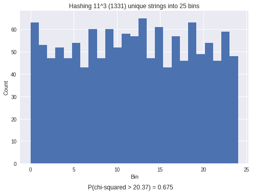
You can see that the chi-squared test results in an insignificant P-value of 0.675, meaning that there is no difference between the observed (generated) indices and the expected uniform distribution. To be thorough, lets look at the resulting P-values for Normal and Uniform random variables.
plt.figure(figsize=(14,5))
plt.subplot(121)
# Normal Distribution
normalX = np.random.normal(0, 10, size=nV)
n, bins, patches = plt.hist(normalX, bins=nBins)
x2, p = ss.chisquare(n)
plt.title("Histogram of %i values from Normal(0, 10) in %i bins"%(nV, nBins))
t=plt.figtext(0.3,0,r'P(chi-squared > %.2f) = %0.3f'%(x2,p), ha='center')

plt.subplot(122)
# Uniform Distribution
uniformX = np.random.uniform(0, 24, size=1400)
n, bins, patches = plt.hist(uniformX, bins=nBins)
x2, p = ss.chisquare(n)
plt.title("Histogram of %i values from Uniform(0, 24) in %i bins"%(nV, nBins))
t=plt.figtext(0.73,0,r'P(chi-squared > %.2f) = %0.3f'%(x2,p), ha='center')
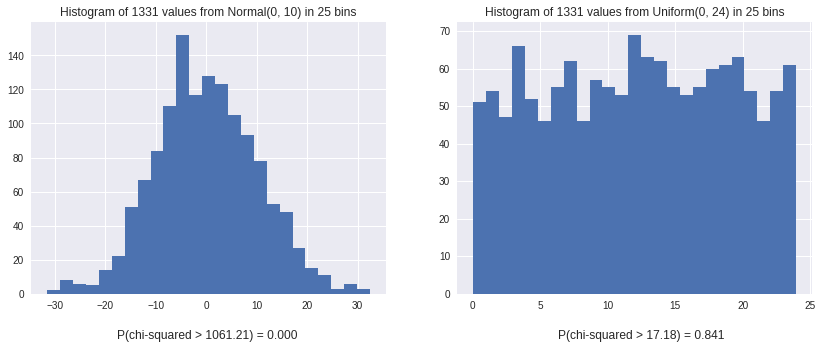
You can see that the Normal distribution has a significant (0.000) P-value, while the Uniform distribution is greater than 0.05. This test will be used to ensure hash functions are correct and look Uniform throughout this post.
XOR Operation
The bitwise XOR operation (^ in python) compares each of the bits in two numbers and outputs the following:
XOR(a, b)
 1. IF a == b RETURN 0
 2. IF a != b RETURN 1
The bitwise XOR operation stands apart from the AND and OR operations because it non-destructively permutes the bits in an input sequence. We can cycle through each number of fixed-bit width to demonstrate
for j in (2,4,8,16):
  bitWidth = j/2
  print "XOR "+' '.join(['%2i'%(x) for x in range(j)])
  for i in range(j):
    print "%2i  "%(i)+' '.join(['%2i'%(i^x) for x in range(j)])
  print

XOR  0  1
 0   0  1
 1   1  0

XOR  0  1  2  3
 0   0  1  2  3
 1   1  0  3  2
 2   2  3  0  1
 3   3  2  1  0

XOR  0  1  2  3  4  5  6  7
 0   0  1  2  3  4  5  6  7
 1   1  0  3  2  5  4  7  6
 2   2  3  0  1  6  7  4  5
 3   3  2  1  0  7  6  5  4
 4   4  5  6  7  0  1  2  3
 5   5  4  7  6  1  0  3  2
 6   6  7  4  5  2  3  0  1
 7   7  6  5  4  3  2  1  0

XOR  0  1  2  3  4  5  6  7  8  9 10 11 12 13 14 15
 0   0  1  2  3  4  5  6  7  8  9 10 11 12 13 14 15
 1   1  0  3  2  5  4  7  6  9  8 11 10 13 12 15 14
 2   2  3  0  1  6  7  4  5 10 11  8  9 14 15 12 13
 3   3  2  1  0  7  6  5  4 11 10  9  8 15 14 13 12
 4   4  5  6  7  0  1  2  3 12 13 14 15  8  9 10 11
 5   5  4  7  6  1  0  3  2 13 12 15 14  9  8 11 10
 6   6  7  4  5  2  3  0  1 14 15 12 13 10 11  8  9
 7   7  6  5  4  3  2  1  0 15 14 13 12 11 10  9  8
 8   8  9 10 11 12 13 14 15  0  1  2  3  4  5  6  7
 9   9  8 11 10 13 12 15 14  1  0  3  2  5  4  7  6
10  10 11  8  9 14 15 12 13  2  3  0  1  6  7  4  5
11  11 10  9  8 15 14 13 12  3  2  1  0  7  6  5  4
12  12 13 14 15  8  9 10 11  4  5  6  7  0  1  2  3
13  13 12 15 14  9  8 11 10  5  4  7  6  1  0  3  2
14  14 15 12 13 10 11  8  9  6  7  4  5  2  3  0  1
15  15 14 13 12 11 10  9  8  7  6  5  4  3  2  1  0
This property is why applying an XOR operation to a random variable results in another random variable. Some hash functions incoroporate the random seed using XOR.
Utilizing XOR
Since Python’s built-in hash() function is random, a NEW random result can be generated by applying the XOR with another number.
Lets see how well this holds up in the real world.
First, lets generate 23^6 strings and hash them into 100 bins.
nBins = 100
choices = 'AGCDEFGHIJKLMNOPQRSTUVWXYZ'
R = 3
nV = len(choices)**R
randomStrings = map(lambda x: ''.join(x), product(choices,repeat=R))
hashValues = map(lambda x: hash(x)%nBins, randomStrings)


# Generate histogram and chi-squared test
plt.figure()
n, bins, patches = plt.hist(hashValues, bins=nBins)
x2, p = ss.chisquare(n)
plt.ylabel("Count")
plt.xlabel("Bin\nP(chi-squared(%i) > %.2f) = %0.3f"%(nBins-1, x2,p))
plt.title("Hashing %i^%i (%i) unique strings into %i bins"%(len(choices), R, nV, nBins))
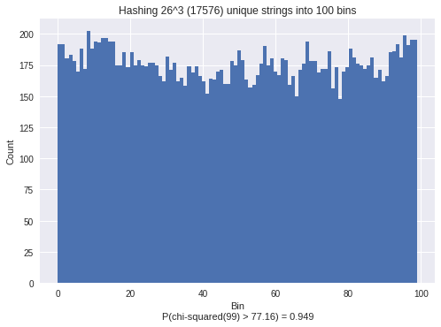
Then, starting from the original hash values, we can generate NEW datasets by applying an XOR with a random variable.
# Generate histogram and chi-squared test
plt.figure(figsize=(15,5))
for i in range(3):
  rI = random.randint(0, 10000)
  modifiedHashValues = map(lambda x: (hash(x)^rI)%nBins, randomStrings)
  plt.subplot(1,3,i+1)
  n, bins, patches = plt.hist(modifiedHashValues, bins=nBins)
  x2, p = ss.chisquare(n)
  plt.xlabel("Bin\nP(chi-squared(%i) > %.2f) = %0.3f"%(nBins-1, x2,p))
  plt.title("Hash values XOR %i into %i bins"%(rI, nBins))
  plt.tight_layout()
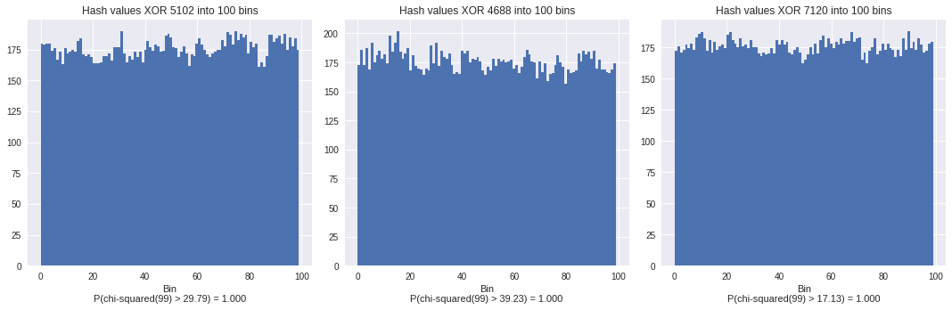
If we did the same with 1000 different random values,
N = 1000
numUniform = 0
for i in range(N):
  rI = random.randint(0, 1000000)
  modifiedHashValues = map(lambda x: (hash(x)^rI)%nBins, randomStrings)
  n, bins = np.histogram(modifiedHashValues, bins=nBins)
  x2, p = ss.chisquare(n)
  if p >= 0.5: numUniform += 1

print "%i/%i = %0.3f XOR'd values were uniform"%(numUniform, N, numUniform/float(N))
661 of the 1000 random datasets would statistically appear to have been generated from a uniform distribution. While not perfect, this is fairly good for a hash function. Please note that since this code uses random values, your results may differ.
edited 2018-02-06
05 Feb 2018